Overview #
Microsoft Excel includes some powerful features for charting and pivot tables, and they can be put to good use in conjunction with Apsona Excel merge. In this document, we will show how to create an Excel template containing a pivot table. The example we will use contains Opportunity data, in which the rows will be the various stages of the opportunities, the columns will be quarters (e.g., Q1-2013), and each cell of the pivot table will contain the sum of the amounts of the opportunities for that stage and quarter. The final result we seek looks like this: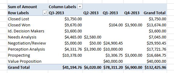
This document assumes that you are familiar with Apsona’s Excel Merge facility.
Creating the template #
The general approach is to create two worksheets in the Excel file, one containing the raw Opportunity data records, and a second containing the pivot table. The pivot table must be set up to get its data from the rows in the raw data worksheet, and since the number of those rows is not known when the template is created, we must use a named range in Excel. Also, the pivot table must be set up to automatically refresh when the file is opened, so that when the user downloads the expanded template, the pivot table is already filled.
Extracting the raw data records #
Create an Excel spreadsheet with a worksheet containing a template for the raw data.
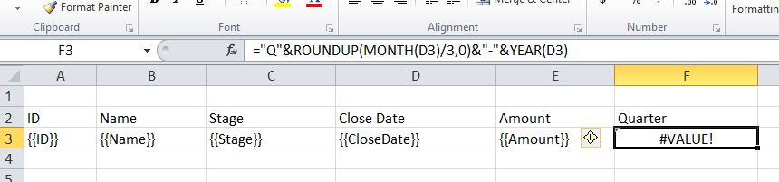
Notice that we have set up the Quarter column as a formula field whose value is derived from the date field. When the template is expanded with the actual data, the formula value will be automatically propagated to all the expanded rows, so that the Quarter cell in each row will contain the correct value associated with that row. The data can be retrieved either directly from the Opportunity object, a simple report or even a multi-step report. The merge feature allows you to merge data from any of those sources.
Setting up a named range #
Define a named range for the table that will contain the expanded Opportunity data, as follows.
- Select the header and template row of the raw data worksheet. In our example, the raw data is in the table range A2:F3, as you can see in the screen shot above. So click cell A2, and then shift-click cell F3 to select the range.
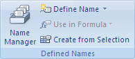
- In Excel 2010, click the Formulas tab of the main menu bar, and then click Name Manager. Alternatively, you can click Ctrl-F3 to bring up the name manager.
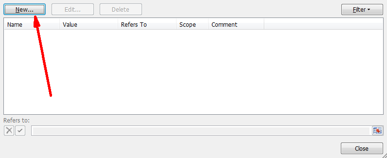
- The name manager popup appears. Click “New” to create a new named range.
- The name definition popup appears. Make up a name for the range, and set up the “Refers to” box as shown.
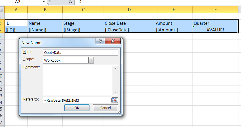
In this example, we have used OpptyData as the name of the range, and the formula used in Refers to isRawData!$A$2:$F$3. So the range refers to the region covered by the two rows of the template, the header row and the template variables row, and the columns spanned by the table. When Apsona fills in the table with the actual data, it will automatically expand the named range so that it refers to the expanded table containing all the actual data rows. - Click Ok to save the range.
- Click Close to close the range manager popup.
Creating the pivot table #
Next, create the pivot table. This must be either in a different worksheet of the Excel file, or above the raw data that is being pivoted. If you try to put the pivot table in the same worksheet under the raw data, the template expander will get confused and the layout will be messed up.
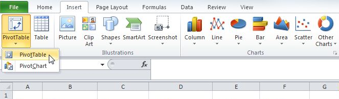
- Create a new worksheet in your Excel file.
- Click inside the worksheet. Then click the Insert tab in the main menu, then PivotTable.
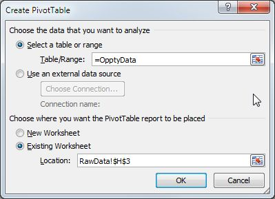
- In the resulting popup, use
=OpptyDataas the name of the table/range, since that is the name we used for the named range. Notice the equals sign beforeOpptyData– that is required to tell Excel that we are using a named range.
- When you click Ok, the pivot table layout editor appears.
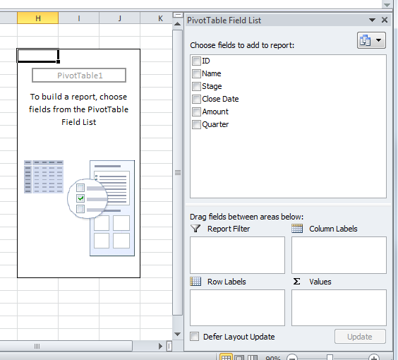
- Drag and drop the Quarter field into the Column Labels area, the Stage into the Row Labels area, and the Amount into the Values area at the bottom right.
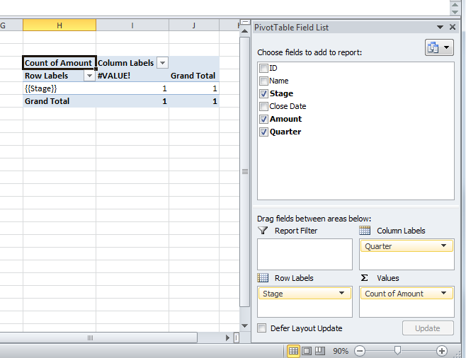
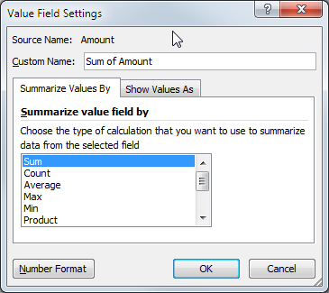
- We are showing the count instead of the sum of the amounts. To remedy this, click the “Count of Amount” label in the Values area and select “Value Field Settings.” In the resulting popup, select “Sum” instead of “Count” in the “Summarize value field by” list. Click Ok.
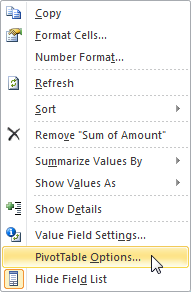
- Click anywhere inside the pivot table area, then right-click, and choose PivotTable Options.
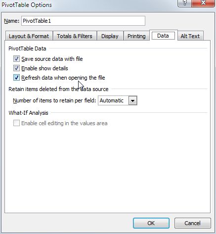
- Click the “Data” tab in the resulting popup, and check the box that says “Refresh data when opening the file.” Click Ok.
- Make sure to change any labels in the pivot table area so that they do NOT include the double-curlies that the Apsona template expander uses. Without this step, Apsona will try to expand the pivot table itself, and the result will be unusable. In this example, Excel has chosen to use
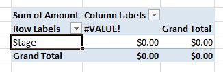
{{Stage}}as the label for the pivot table row, and we have changed it toStage. You can make up any name you want, because Excel will automatically re-fill the pivot table when the template is expanded. Type F2 to edit the field, and change it to whatever you want.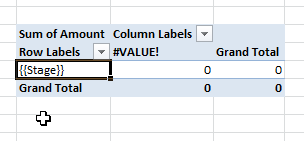
Finishing up #
Save the resulting template, Upload the template to your Salesforce Document object, and use it as the template when expanding your Opportunity data.